Conjugate heat transfer

At the end of this you will have a case that solves the flow and the temperature in a fluid and the conduction in a solid at the same time, coupled at the faces they share, with the heat crossing between them rather than stopping at a boundary condition you invented.

This needs a paid licence, for two separate reasons. Conjugate Heat Transfer is not one of the analysis types the free tier allows, and a conjugate case is a multi-region case, which the free tier’s cell-zone gate also blocks. Both appear on the Problems tab as errors before you run, naming the tier and what it allows. On the free tier the case is safe to build and look at; it will not solve.

One thing in this workflow is not finished. The box that positions a solid region is stored on the region and written to topoSetDict, but the Materials pane provides no control for it, so a solid region cannot be placed from the interface in this build. Read Placing the solid before you plan a real case around this.

Before you start

Read Flow in a pipe — a conjugate case is usually an internal-flow case with a wall that conducts, and everything about meshing and wall treatment carries over.

What makes this different

Every other tutorial solves one mesh. A conjugate case solves several.

The application meshes the whole thing as one mesh, then cuts it into regions along cell zones using splitMeshRegions, and hands each region to the solver with coupled conditions generated on the faces where two regions meet. That is why the run pipeline for a conjugate case has a step the others do not, and why cell zones are the licensed feature that gates it.

The consequence you have to plan for: a region only exists if there is a cell zone to cut it out of. Declaring a region in a list is not enough.

1. Create the case

Press New case. In the Create Simulation dialog choose Heat Transfer, then Conjugate (CHT).

The right-hand panel lists what this covers — fluid plus solid regions, interface coupling, radiation, steady or transient — and what it does not: multiphase and combustion.

The review page is worth reading here rather than skipping. For a conjugate case it inserts an extra line into SET UP NEXT: Advanced concepts, described as “the solid regions, which the mesh is split along”. The wizard is telling you in advance that this case has a step the others do not.

The wizard derives chtMultiRegionFoam, or its steady counterpart if you set Time dependency to Steady-state under Models.

2. Geometry

Select Geometry and import the assembly, or leave it empty if the solid is a simple block inside a box of fluid.

If your CAD has the fluid and the solid as separate bodies, press Split into parts so each becomes its own patch. That is what lets you set a different condition on the outside of the solid from the one on the fluid inlet.

3. Mesh

Select Mesh and mesh as you normally would. The mesh at this stage is a single mesh covering everything — fluid and solid alike. It is cut afterwards.

Two things to get right, because they are harder to fix later:

Resolve the interface. The faces where the solid meets the fluid are where the whole answer is decided, and a coarse mesh there gives a coupled boundary condition very little to work with. If the solid is an imported surface, use Refinements to raise the surface level on it.

Do not skip boundary layers on the fluid side. The heat transfer coefficient at a wall is a boundary-layer quantity. The Boundary layers pane and its y+ target behave exactly as in the other tutorials, and the same rule applies: Target y+ must agree with Wall treatment under Models.

Press Generate mesh, then check Quality as usual.

4. Models

Select Models.

Analysis type reads Conjugate Heat Transfer. Two toggles under Physics are already on and should stay on:

• Energy equation — obviously, since temperature is the point.
• Gravity / buoyancy — less obviously. A conjugate solver carries gravity as a matter of course, and turning it off does not make the case cheaper, it makes it wrong. Heat moving through a fluid moves it, and buoyancy is how.

Leave Model at k-omega SST and Wall treatment on Wall functions unless the mesh supports better.

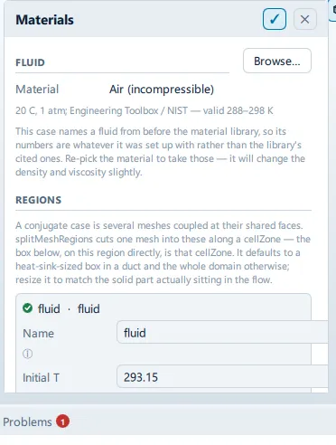
5. Materials — the regions

Select Materials. Below the fluid properties there is a Regions section that only appears for a multi-region case.

The pane states the mechanism plainly:

A conjugate case is several meshes coupled at their shared faces. splitMeshRegions cuts one mesh into these along its cellZones, so every solid region below needs a matching cellZone.

Two regions are there to begin with, fluid and solid. Each carries:

• Name — and its hint is the important part: “Must match the cellZone the mesh carries — that is what splitMeshRegions names the region after.” The region name is not a label. It is the key that ties the declaration to the mesh.
• Initial T — where that region starts.

A solid region carries three more:

• Material — a name, for the report.
• Density and Cp — the thermal mass, which is what decides how long a transient takes to settle. They do nothing at all in a steady run.
• Conductivity — isotropic and constant. The hint gives the scale: steel about 45, aluminium about 200, a typical plastic about 0.2. Three orders of magnitude across ordinary engineering materials, so this is not a field to leave at its default.

+ Fluid region and + Solid region add more.

Placing the solid, and the limit you will hit

Each region carries a box that says which cells belong to it, and that box is what topoSetDict cuts the zone from. The Materials pane does not render a control for it.

The consequences are specific and worth knowing before you commit to a case:

• The two regions that come with a new conjugate case have a box already set, and a case built on those two will validate and run.
• A region added with + Solid region is created spanning the entire domain. The Problems tab reports it immediately — “The solid region … covers the whole domain, so there would be no fluid left. Give it a box or sphere inside the domain.” — and there is nowhere in the interface to give it one.

So: build conjugate cases on the two regions the analysis type provides. If you need a third, the case file can be edited outside the application, but that is not a workflow this manual is going to teach.

6. Advanced concepts

Select Advanced concepts.

For a conjugate case the region zones are generated for you from the region list, so you do not need to add anything here to make the split happen — despite what the Materials text suggests.

What this node is genuinely for in a thermal case is Heat sources. Add one with the + beside that category and you get an item with its own tree node and editor, offering:

• Volumetric heat source with a Power in watts — a component dissipating into the solid it sits in.
• Fixed temperature — a region held at a temperature.
• Heat exchanger — likewise, with a temperature.

Every one of them acts on a Cell zone, and the item’s Zone geometry section is where that zone is defined: Shape as box, cylinder or sphere, with the corresponding min and max, radius, length and axis fields, plus a Fit to geometry button. Note the difference from the region list above — here the geometry is editable.

If the energy equation is off, the pane says so: “a heat source has nothing to act on”.

7. Initial conditions

Select Initial conditions and set Temperature.

A conjugate case is sensitive to this in a way an isothermal one is not. A solid started at the fluid temperature has no heat in it and takes the whole run to acquire any; a solid started far from equilibrium spends the run coming back. Start near where you expect to end.

8. Boundary conditions

Select Boundary conditions.

The condition to know here is Thermal wall. A plain Wall is adiabatic for the energy equation; a Thermal wall takes a Temperature. Use it on the outside surfaces of the solid, where you know the environment.

You do not set a condition on the interface between the regions. That is the whole point of solving them conjugately: the coupling is generated on the shared faces, and heat crosses rather than stopping at a number you supplied. If you find yourself wanting to specify a wall temperature on the solid–fluid boundary, you are setting up the case you were trying to avoid.

Select any patch and check the This writes block at the bottom of the pane. On a conjugate case it lists a temperature entry alongside the flow fields — that is the one to sanity-check.

9. Result control

Select Result control and press + Wall heat flux. Its description says why it is here: “heat into or out of a wall, W and W/m2 - the answer a thermal case is run for”.

Add + Field minimum and maximum as well. On a thermal case the peak solid temperature is usually the thing that decides whether the design passes, and this reports the extremes of each field and where they are.

+ Patch data with Operation set to areaAverage on a T field gives you the mean temperature of a surface, which is what most thermal specifications are written against.

10. Simulation control and run

A steady conjugate run reaches equilibrium; a transient one shows you how long it takes to get there. Choose deliberately — thermal mass only matters in the second.

Select Runs and press Start run.

Watch Residuals. A conjugate case has more equations than a flow case and they converge at different rates; the energy residual typically lags the pressure one, and that is normal.

Watch Monitors for the wall heat flux. That is the convergence test that matters. A thermal case whose residuals have fallen but whose heat flux is still drifting has not settled — heat is still filling the solid.

11. Post-processing

Select Post-processing and press Show results.

Under Ready-made views, press Temperature and heat. It builds a slice and a surface, both coloured by temperature: “where the heat is, and what the solid is being asked to carry”.

The thing to look for is continuity of temperature across the interface with a discontinuity in gradient. Temperature is continuous; its slope is not, because the conductivities differ. If temperature itself jumps across the interface, the regions are not coupled and you are looking at two independent solutions displayed side by side.

12. Report

Select Report. Keep Physics and materials on so the conductivities are recorded — a thermal result is not reviewable without them — and Results and field ranges for the peak temperatures.

What you should see

A temperature field that is continuous across the solid–fluid interface and changes slope there. A heat flux that stopped drifting before the run ended. A peak solid temperature you can defend.

Signs it is wrong: two regions at obviously unrelated temperatures (they were not coupled — check that the region names match what the mesh was cut into), a solid at exactly its initial temperature everywhere (no heat is reaching it), or a run that never started because the region zone covered the whole domain.

What to try next

• Flow in a pipe — the fluid half of this on its own, which is worth running first when a conjugate case misbehaves. Half a case that works is a better diagnostic than a whole one that does not.
• Mesh independence study — heat transfer coefficients are more mesh-sensitive than drag is, not less.
• Rotating machinery with MRF for the other cell-zone workflow in the application.