
Flow over a cylinder
At the end of this you will have a two-dimensional transient run of flow past a circular cylinder, with a shed wake you can watch in the viewport and a lift coefficient that oscillates in the Monitors tab.
This is the first tutorial because the answer checks itself. Above a Reynolds number of a few tens the wake behind a cylinder sheds alternately, and lift oscillates about zero while drag stays roughly steady. If your wake sits still and symmetric, something is wrong, and you do not need a plot to see it.
Runs on the free tier. The analysis type is Incompressible, which the free tier allows, and a two-dimensional mesh comfortably fits the 250,000-cell cap — it is one cell thick, so it costs roughly a hundredth of the equivalent 3-D mesh.
Before you start
Section titled “Before you start”Read Your first simulation. This tutorial assumes you know what the setup tree is and where the bottom dock lives.
You need to supply one file. The application imports geometry; it does not draw it, and no cylinder ships with it. Six demo bodies do — a streamlined hull, an impeller, an inclined plate, an obstacle lattice, a sphere and a cantilever bar — but which one a case gets is derived from its physics rather than chosen, and the route to the hull is Worked example on the home screen. Export a cylinder from whatever CAD you use, as STL or OBJ, extruded along x. The extruded length does not matter much — the 2-D mesh collapses that direction to a single cell — so make it comparable to the diameter and centre it near the origin.
Where the commands are
Section titled “Where the commands are”Two places, and this tutorial names both. The setup tree down the left is the case: selecting a row opens its pane beside it, and every “Select X” below means that row. Commands live on the ribbon across the top, in three tabs — Model, Geometry, Results — with the commands in labelled groups. On the Model tab: Generate mesh and Quality are in MESH, Start run and Continue are in RUN, Comparison and Report are in STUDY. Selecting a Post-processing row switches the ribbon to the Results tab by itself.
1. Create the case
Section titled “1. Create the case”From the home screen, press New case. The Create Simulation dialog opens on the physics drill-down.
Choose Single Phase, then Low Speed, then Transient (PIMPLE), pressing Next to go down each level. The right-hand panel says what each choice covers before you commit to it, and Next on the last one takes you to a review page listing what the case will derive and what you still have to set.
The wizard derives pimpleFoam. Shedding is unsteady, so a steady solver is the
wrong tool here — it will grind towards a symmetric answer that does not exist.
There is also a Transient (PISO) leaf; PIMPLE is used here because the
adjustable time step in Simulation control is built around it.
Give the simulation a name under NAME on the review page, then press Create simulation. Inside an existing case the same button reads Add simulation.
2. Geometry
Section titled “2. Geometry”Select Geometry — the row at the very top of the tree, above the simulation heading. There are two rows called Geometry: that one, which belongs to the case, and one under the simulation, which only chooses which of the case’s bodies this simulation runs on. Import lives on the case’s row, and so does everything else in this section.
Press Import geometry. Pick your cylinder file.
Check Units matches what the file is in — geometry is rescaled to metres on import, and a cylinder exported in millimetres and left as one solves a body a thousand times too big.
Then read the Geometry info block. Size should be the cylinder you
expect. Watertight should say yes; if it says open edges, snappyHexMesh
will still mesh it but the surface has holes, and holes are where a mesh leaks
into the inside of a body.
3. Mesh
Section titled “3. Mesh”Select Mesh.
Leave Mesher on snappyHexMesh (hex-dominant) — there is a body to wrap a mesh around.
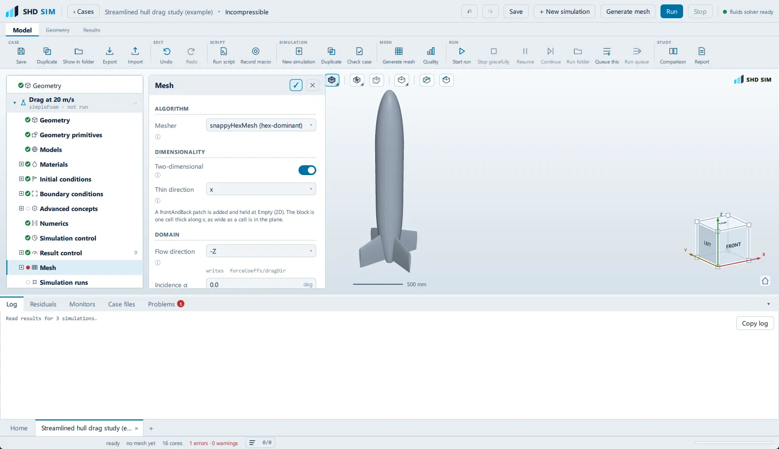
Under Dimensionality, turn on Two-dimensional and set Thin direction
to x, the axis you extruded along. A frontAndBack patch appears in the
tree under Boundary conditions, held at Empty (2D). That patch is not a
boundary condition; it is the statement that the direction is not solved.
Leave Flow direction at its default, −Z. It must not be the thin direction, and here it is not.
Leave Auto wind tunnel on. It sizes the background block from the geometry bounding box in multiples of body length, and the five pads are those multiples. Each label carries its axis in brackets — Ahead, Wake, Sides, Above, Below, each followed by the signed axis it pads along, derived from the flow direction — so you never have to work out which way round they are. The wake pad is the largest by default, which is right: everything interesting happens downstream.
Now look at the estimate block near Generate. It reads
Estimate: … M cells, with Current mesh: … M cells on the line below it, and
if the estimate exceeds the budget it says so in amber.
4. Refinements
Section titled “4. Refinements”Select Refinements.
The one setting that matters on the free tier is Max cells. It defaults to 2,000,000, which is eight times the free cap, so the Problems tab will refuse the run before you ever reach it. Set Max cells to 250000 or below.
Then bring the estimate down until it fits. Two levers, in order of effect:
Raise Base cell size under Mesh — or press Suggest from domain there to get a size scaled to the box. Then reduce Level max here if you are still over. The → base … surface … block in this pane shows both cell sizes and the running estimate as you type.
Watch the Problems tab as you go. The cell-cap error names the estimate and the limit, so you can tell whether you are close or nowhere near.
5. Boundary layers
Section titled “5. Boundary layers”Select Boundary layers.
Leave Target y+ at 30 and Wall treatment — under Models — at Wall functions. Wall functions want y+ between 30 and 300, and the pane says so; resolving the boundary layer instead would need y+ near 1, and a mesh that fine will not fit in 250,000 cells even in two dimensions.
The block at the top reports the Reynolds number the case is at, the first-layer height that y+ implies, and the total stack thickness. If the amber warning appears saying the stack is as thick as the surface cell, reduce Layers or Expansion until it clears — a layer stack thicker than the cell it sits inside is a mesh that will not build cleanly.
6. Generate the mesh, then check it
Section titled “6. Generate the mesh, then check it”Press Generate mesh — on the pane, or in the ribbon’s MESH group on the Model tab. Watch the Log tab.
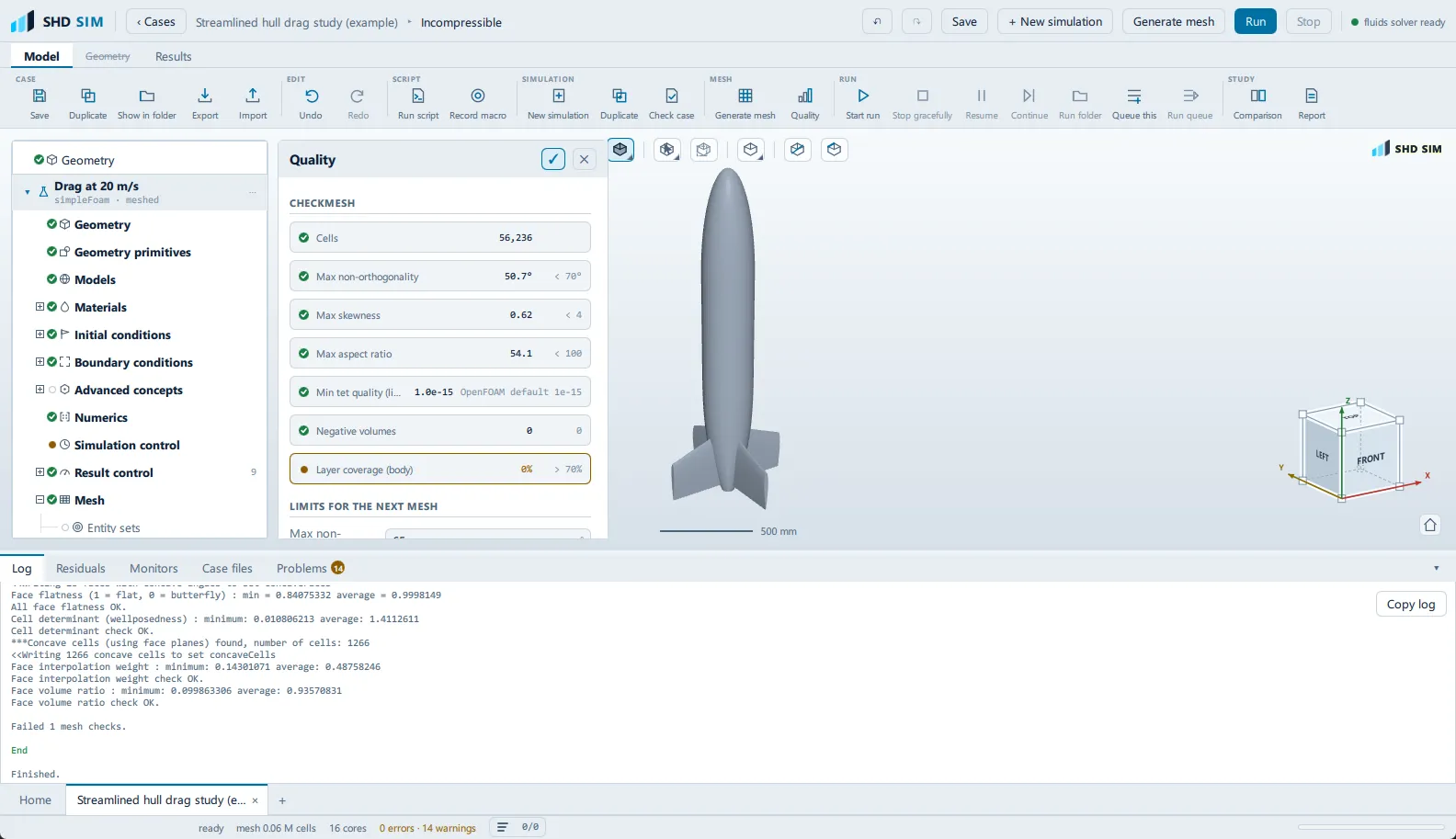
When it finishes, select Quality, which is under Mesh in the tree rather than beside it. Seven rows, five of them a measurement against a stated limit:
- Cells is the count, and it has no limit column. It is there to be read, not judged.
- Max non-orthogonality, limit
< 70°. Between 60 and 70 you get a recommendation with an Apply to numerics button, which sets the snGrad scheme and the non-orthogonal correctors for you. Take it. - Max skewness, limit
< 4. - Max aspect ratio, limit
< 100. - Min tet quality (limit) is the odd one out and says so in its own name: it
is what snappyHexMesh was allowed to produce, not something checkMesh
measured, because checkMesh reports no minimum tet quality at all. Its limit
column reads
OpenFOAM default 1e-15. - Negative volumes must be
0. Anything else means the mesh is broken and no solver will produce sense from it. - Layer coverage (body), limit
> 70%. Below that there is an Apply to mesh settings button, which relaxes the layer controls; re-mesh afterwards.
7. Models, Materials, Initial conditions
Section titled “7. Models, Materials, Initial conditions”Models should already read Incompressible, Transient, PIMPLE, with Model at k-omega SST. Leave it. The Derived block at the bottom shows the solver and the field set the case will write.
Materials defaults to Air (incompressible). The derived block shows the Reynolds number this fluid gives at the reference velocity and length — worth a glance, because it is the number that decides whether you get shedding at all.
Initial conditions defaults to Uniform with Track the inlet on, so the domain starts at the inlet velocity rather than at rest. Leave it. A transient case started from rest spends its first physical seconds establishing the flow, and the pane warns you when that is what you have asked for.
8. Boundary conditions
Section titled “8. Boundary conditions”Select Boundary conditions. Five patches, already assigned:
| Patch | Type | |
|---|---|---|
inlet |
Velocity inlet | 10 m/s |
outlet |
Pressure outlet | 0 Pa gauge |
body |
Wall | the cylinder |
farfield |
Far field | the sides |
frontAndBack |
Empty (2D) | added by the 2-D toggle |
You do not need to change any of them. Select inlet and look at the
This writes block at the bottom of the pane: one boundary condition entry
per field, generated from the single choice Velocity inlet. That fan-out is
the thing the application is doing for you.
9. Result control
Section titled “9. Result control”Select Result control and press + Force coefficients.
Set Patch to body. Leave References from the case on — it takes the
frontal area, the model length and the inlet speed from the geometry and the
boundary conditions rather than making you retype them.
This is the item that makes the answer checkable. Without it you will have a picture; with it you will have Cl against time, which is what says the wake is shedding.
Add + y+ as well. It writes y+ on the walls so you can confirm afterwards that the wall treatment was being asked for something it can do.
10. Simulation control
Section titled “10. Simulation control”Select Simulation control.
End time and Time step define the run; the block underneath tells you how many time steps that is at the starting Δt and how many times it will write. Adjust time step to Courant number is on by default, with Max Courant at 1 for an incompressible case, so the step is set by the flow rather than by your guess.
You need enough end time for several shedding cycles — one cycle is roughly the time the flow takes to travel a few diameters. Start with the default, watch the lift monitor, and extend it if the oscillation has not established.
On the free tier the Cores list is one entry long. It is a ladder rather than a typed number, and the licence shortens the ladder, so there is nothing to pick that the licence would then refuse. Its hint says what that costs: the run still completes, on one core, and takes longer.
11. Run
Section titled “11. Run”Select Simulation runs — that is the node’s name; there is no row called Runs — and press Start run. The same command is in the ribbon’s RUN group on the Model tab, and the top bar’s Run button does it too, opening the bottom dock for you: on Residuals if the case is clean, on Problems if it is not.
What to watch, in the bottom dock:
- Residuals should fall within each time step and stay bounded across them. A transient run does not converge to a flat line the way a steady one does.
- Monitors is where the answer appears. Cd settles to a roughly constant value; Cl starts near zero, then grows into a regular oscillation about zero. That oscillation is the shedding.
- Log shows the Courant number. If it is being clipped hard every step, the time step is fighting the flow.
If Cl stays flat at zero for the whole run, the wake has not tripped. Give it more end time first; a perfectly symmetric mesh and a perfectly symmetric initial field can take a while to fall off the knife edge.
12. Post-processing
Section titled “12. Post-processing”Post-processing is not a step beside the setup. It hangs under the run, at
Simulation runs → <your run> → Post-processing, and it appears only once that
run has finished — a study with three runs has three of them, and one hung off
the study could not say which run it meant. Select it and the ribbon switches to
the Results tab by itself.
Press Show results.
The fastest route to the picture is under Ready-made views: press Wake and vortices, which builds a surface, a vorticity threshold named “Vortex cores”, and streamlines. Step through the written times with the time controls and the shed vortices march downstream.
If you would rather build it yourself, a Slice through the middle coloured by velocity is the single most useful view. Filters are added from the Results ribbon’s FILTERS group rather than from the pane; the pane lists what the pipeline already holds.
13. Report
Section titled “13. Report”Select Report, which sits under the same run as Post-processing did. Tick the sections you want and press Export PDF (A4). On the free tier it carries a watermark; everything in it is real.
What you should see
Section titled “What you should see”A wake that sheds. Vortices leaving alternate sides of the cylinder and travelling downstream in two staggered rows, and a lift coefficient oscillating about zero at a steady frequency and amplitude. Drag oscillates too, at twice the lift frequency and much more weakly.
A symmetric, stationary wake means one of three things: the run has not gone on long enough, the Reynolds number is too low for shedding, or the case is being solved steady. Check Models shows Transient before you look anywhere else.
What to try next
Section titled “What to try next”- Mesh independence study uses this exact case and asks whether the answer you just got is a property of the flow or of your mesh. It is the natural second step and the one that turns a picture into a result.
- Flow in a pipe for the internal-flow half of the workflow, where there is no body and the mesh is just the domain.
- External aerodynamics for the same workflow in three dimensions, with refinement regions and a drag split.